Riemann integral
In the branch of mathematics known as real analysis, the Riemann integral, created by Bernhard Riemann, was the first rigorous definition of the integral of a function on an interval. While the Riemann integral is unsuitable for many theoretical purposes, it is one of the easiest integrals to define. For a great many functions and practical applications, the Riemann integral can also be readily evaluated by using the fundamental theorem of calculus or (approximately) by numerical integration.
Some of the technical deficiencies in Riemann integration can be remedied by the Riemann–Stieltjes integral, and most of these disappear with the Lebesgue integral, which is of theoretical interest only, and not in applied mathematics.
Contents |
Overview
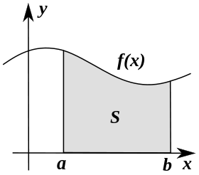
Let  be a non-negative real-valued function of the interval
 ![[a,b]](/I/2c3d331bc98b44e71cb2aae9edadca7e.png) , and let
, and let  be the region of the plane under the graph of the function and above the interval (see the figure on the top right). We are interested in measuring the area of
  . Once we have measured it, we will denote the area by:

The basic idea of the Riemann integral is to use very simple approximations for the area of . By taking better and better approximations, we can say that "in the limit" we get exactly the area of under the curve.
Note that where ƒ can be both positive and negative, the integral corresponds to signed area under the graph of ƒ; that is, the area above the x-axis minus the area below the x-axis.
Definition
Partitions of an interval
A partition of an interval is a finite sequence  . Each
 ![[x_i, x_{i+1}]](/I/38d37ec1a65c2b21ca226c22a611631d.png) is called a subinterval of the partition. The mesh of a partition is defined to be the length of the longest subinterval , that is, it is
is called a subinterval of the partition. The mesh of a partition is defined to be the length of the longest subinterval , that is, it is 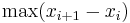 where
where  . It is also called the norm of the partition.
A tagged partition of an interval is a partition of an interval together with a finite sequence of numbers  subject to the conditions that for each
  ,
,  . In other words, it is a partition together with a distinguished point of every subinterval. The mesh of a tagged partition is the same as that of an ordinary partition.
Suppose that  together with are a tagged partition of , and that
  together with
  are another tagged partition of . We say that and together are a refinement of together with if for each integer with
  , there is an integer
  such that
  and such that
  for some
  with
with  . (It is not correct to allow to equal
  because
  is greater than or equal to
  .) Said more simply, a refinement of a tagged partition takes the starting partition and adds more tags, but does not take any away.
We can define a partial order on the set of all tagged partitions by saying that one tagged partition is bigger than another if the bigger one is a refinement of the smaller one.
Riemann sums
Choose a real-valued function which is defined on the interval . The Riemann sum of with respect to the tagged partition together with is:
Each term in the sum is the product of the value of the function at a given point, and the length of an interval. Consequently, each term represents the area of a rectangle with height  and length
  . The Riemann sum is the signed area under all the rectangles.
Riemann integral
Loosely speaking, the Riemann integral is the limit of the Riemann sums of a function as the partitions get finer. If the limit exists then the function is said to be integrable (or more specifically Riemann-integrable). The Riemann sum can be made as close as desired to the Riemann integral by making the partition fine enough.
One important fact is that the mesh of the partitions must become smaller and smaller, so that in the limit, it is zero. If this were not so, then we would not be getting a good approximation to the function on certain subintervals. In fact, this is enough to define an integral. To be specific, we say that the Riemann integral of ƒ equals s if the following condition holds:
- For all ε > 0, there exists δ > 0 such that for any tagged partition and whose mesh is less than δ, we have
However, there is an unfortunate problem with this definition: it is very difficult to work with. So we will make an alternate definition of the Riemann integral which is easier to work with, then prove that it is the same as the definition we have just made. Our new definition says that the Riemann integral of ƒ equals s if the following condition holds:
- For all ε > 0, there exists a tagged partition and such that for any refinement and of and , we have
Both of these mean that eventually, the Riemann sum of ƒ with respect to any partition gets trapped close to s. Since this is true no matter how close we demand the sums be trapped, we say that the Riemann sums converge to s. These definitions are actually a special case of a more general concept, a net.
As we stated earlier, these two definitions are equivalent. In other words, s works in the first definition if and only if s works in the second definition. To show that the first definition implies the second, start with an ε, and choose a δ that satisfies the condition. Choose any tagged partition whose mesh is less than δ. Its Riemann sum is within ε of s, and any refinement of this partition will also have mesh less than δ, so the Riemann sum of the refinement will also be within ε of s. To show that the second definition implies the first, it is easiest to use the Darboux integral. First one shows that the second definition is equivalent to the definition of the Darboux integral; for this see the page on Darboux integration. Now we will show that a Darboux integrable function satisfies the first definition. Fix ε, and choose a partition such that the lower and upper Darboux sums with respect to this partition are within ε/2 of the value s of the Darboux integral. Let r equal the supremum of |ƒ(x)| on [a,b]. If r = 0, then ƒ is the zero function, which is clearly both Darboux and Riemann integrable with integral zero. Therefore we will assume that r > 0. If m > 1, then we choose δ to be less than both ε/2r(m − 1) and  . If m = 1, then we choose δ to be less than one. Choose a tagged partition and . We must show that the Riemann sum is within ε of s.
To see this, choose an interval [xi, xi + 1]. If this interval is contained within some [yj, yj + 1], then the value of ƒ(ti) is between mj, the infimum of ƒ on [yj, yj + 1], and Mj, the supremum of ƒ on [yj, yj + 1]. If all intervals had this property, then this would conclude the proof, because each term in the Riemann sum would be bounded a corresponding term in the Darboux sums, and we chose the Darboux sums to be near s. This is the case when m = 1, so the proof is finished in that case. Therefore we may assume that m > 1. In this case, it is possible that one of the [xi, xi + 1] is not contained in any [yj, yj + 1]. Instead, it may stretch across two of the intervals determined by . (It cannot meet three intervals because δ is assumed to be smaller than the length of any one interval.) In symbols, it may happen that

(We may assume that all the inequalities are strict because otherwise we are in the previous case by our assumption on the length of δ.) This can happen at most m − 1 times. To handle this case, we will estimate the difference between the Riemann sum and the Darboux sum by subdividing the partition at yj + 1. The term ƒ(ti)(xi − xi + 1) in the Riemann sum splits into two terms:

Suppose that ti ∈ [xi, xi + 1]. Then mj ≤ ƒ(ti) ≤ Mj, so this term is bounded by the corresponding term in the Darboux sum for yj. To bound the other term, notice that yj + 1 − xi + 1 is smaller than δ, and δ is chosen to be smaller than ε/2r(m − 1), where r is the supremum of |ƒ(x)|. It follows that the second term is smaller than ε/2(m − 1). Since this happens at most m − 1 times, the total of all the terms which are not bounded by the Darboux sum is at most ε/2. Therefore the distance between the Riemann sum and s is at most ε.
Examples
Let ![f:[0,1] \rightarrow \mathbb{R}](/I/ea78d31a30bd943ad155434a476207fb.png) be the function which takes the value 1 at every point. Any Riemann sum of on
be the function which takes the value 1 at every point. Any Riemann sum of on ![[0,1]](/I/ccfcd347d0bf65dc77afe01a3306a96b.png) will have the value 1, therefore the Riemann integral of on is 1.
will have the value 1, therefore the Riemann integral of on is 1.
Let ![I_{\mathbb{Q}}:[0,1] \rightarrow \mathbb{R}](/I/77d461bdb83f087b7109a78d129c4abf.png) be the indicator function of the rational numbers in ; that is,
be the indicator function of the rational numbers in ; that is,  takes the value 1 on rational numbers and 0 on irrational numbers. This function does not have a Riemann integral. To prove this, we will show how to construct tagged partitions whose Riemann sums get arbitrarily close to both zero and one.
To start, let and be a tagged partition (each  is between
  and ). Choose
  . The have already been chosen, and we can't change the value of at those points. But if we cut the partition into tiny pieces around each , we can minimize the effect of the . Then, by carefully choosing the new tags, we can make the value of the Riemann sum turn out to be within
  of either zero or one—our choice!
Our first step is to cut up the partition. There are  of the , and we want their total effect to be less than . If we confine each of them to an interval of length less than
  , then the contribution of each to the Riemann sum will be at least
  and at most
  . This makes the total sum at least zero and at most . So let
  be a positive number less than . If it happens that two of the are within of each other, choose smaller. If it happens that some is within of some
  , and is not equal to , choose smaller. Since there are only finitely many and , we can always choose sufficiently small.
Now we add two cuts to the partition for each . One of the cuts will be at  , and the other will be at
  . If one of these leaves the interval , then we leave it out. will be the tag corresponding to the subinterval
 ![[t_i - \delta/2,t_i + \delta/2]](/I/859136a2616733d80aeb21d1233a3c61.png) . If is directly on top of one of the , then we let be the tag for both
. If is directly on top of one of the , then we let be the tag for both ![[t_i - \delta/2,x_j]](/I/3729ee9a3145b7c244c03de6bae5c98a.png) and
and ![[x_j,t_i + \delta/2]](/I/cb852930981a295c0f761a5c796eca2c.png) . We still have to choose tags for the other subintervals. We will choose them in two different ways. The first way is to always choose a rational point, so that the Riemann sum is as large as possible. This will make the value of the Riemann sum at least
. We still have to choose tags for the other subintervals. We will choose them in two different ways. The first way is to always choose a rational point, so that the Riemann sum is as large as possible. This will make the value of the Riemann sum at least  . The second way is to always choose an irrational point, so that the Riemann sum is as small as possible. This will make the value of the Riemann sum at most .
Since we started from an arbitrary partition and ended up as close as we wanted to either zero or one, it is false to say that we are eventually trapped near some number  , so this function is not Riemann integrable. However, it is Lebesgue integrable. In the Lebesgue sense its integral is zero, since the function is zero almost everywhere. But this is a fact that is beyond the reach of the Riemann integral.
There are even worse examples. is equivalent (that is, equal almost everywhere) to a Riemann integrable function, but there are non-Riemann integrable bounded functions which are not equivalent to any Riemann integrable function. For example, let C be the Smith–Volterra–Cantor set, and let IC be its indicator function. Because C is not Jordan measurable, IC is not Riemann integrable. Moreover, no function g equivalent to IC is Riemann integrable: g, like IC, must be zero on a dense set, so as in the previous example, any Riemann sum of g has a refinement which is within ε of 0 for any positive number ε. But if the Riemann integral of g exists, then it must equal the Lebesgue integral of IC, which is 1/2. Therefore g is not Riemann integrable.
Similar concepts
It is popular to define the Riemann integral as the Darboux integral. This is because the Darboux integral is technically simpler and because a function is Riemann-integrable if and only if it is Darboux-integrable.
Some calculus books do not use general tagged partitions, but limit themselves to specific types of tagged partitions. If the type of partition is limited too much, some non-integrable functions may appear to be integrable.
One popular restriction is the use of "left-hand" and "right-hand" Riemann sums. In a left-hand Riemann sum,  for all , and in a right-hand Riemann sum,
  for all . Alone this restriction does not impose a problem: we can refine any partition in a way that makes it a left-hand or right-hand sum by subdividing it at each . In more formal language, the set of all left-hand Riemann sums and the set of all right-hand Riemann sums is cofinal in the set of all tagged partitions.
Another popular restriction is the use of regular subdivisions of an interval. For example, the  th regular subdivision of consists of the intervals
 ![[0, 1/n], [1/n, 2/n], \ldots, [(n-1)/n, 1]](/I/70045082bf22ffe3b478efeafe9c5fe5.png) . Again, alone this restriction does not impose a problem, but the reasoning required to see this fact is more difficult than in the case of left-hand and right-hand Riemann sums.
. Again, alone this restriction does not impose a problem, but the reasoning required to see this fact is more difficult than in the case of left-hand and right-hand Riemann sums.
However, combining these restrictions, so that one uses only left-hand or right-hand Riemann sums on regularly divided intervals, is dangerous. If a function is known in advance to be Riemann integrable, then this technique will give the correct value of the integral. But under these conditions the indicator function will appear to be integrable on with integral equal to one: Every endpoint of every subinterval will be a rational number, so the function will always be evaluated at rational numbers, and hence it will appear to always equal one. The problem with this definition becomes apparent when we try to split the integral into two pieces. The following equation ought to hold:
If we use regular subdivisions and left-hand or right-hand Riemann sums, then the two terms on the left are equal to zero, since every endpoint except 0 and 1 will be irrational, but as we have seen the term on the right will equal 1.
As defined above, the Riemann integral avoids this problem by refusing to integrate . The Lebesgue integral is defined in such a way that all these integrals are 0.
Properties
The Riemann integral is a linear transformation; that is, if and  are Riemann-integrable on and
  and
and  are constants, then
Because the Riemann integral of a function is a number, this makes the Riemann integral a linear functional on the vector space of Riemann-integrable functions. It can be shown that a real-valued function on is Riemann-integrable if and only if it is bounded and continuous almost everywhere in the sense of Lebesgue measure.
If a real-valued function on is Riemann-integrable, it is Lebesgue-integrable.
If  is a uniformly convergent sequence on with limit , then Riemann integrability of all implies Riemann integrability of , and
If a real-valued function is monotone on the interval ![[a,b],](/I/f12644f1c0d00b07716732c25819450c.png) it is Riemann-integrable, since its set of discontinuities is denumerable, and therefore of Lebesgue measure zero.
it is Riemann-integrable, since its set of discontinuities is denumerable, and therefore of Lebesgue measure zero.
An indicator function of a bounded set is Riemann-integrable if and only if the set is Jordan measurable.[1]
Lebesgue's criterion for Riemann integrability:[1] A function on a compact interval is Riemann integrable if and only it is bounded and the set of its points of discontinuity has measure zero.
Generalizations
It is easy to extend the Riemann integral to functions with values in the Euclidean vector space Rn for any n. The integral is defined by linearity; in other words, if ƒ = (ƒ1,…,ƒn) then
In particular, since the complex numbers are a real vector space, this allows the integration of complex valued functions.
The Riemann integral is only defined on bounded intervals, and it does not extend well to unbounded intervals. The simplest possible extension is to define such an integral as a limit, in other words, as an improper integral. We could set:

Unfortunately, this does not work well. Translation invariance, the fact that the Riemann integral of the function should not change if we move the function left or right, is lost. For example, let ƒ(x) = −1 for all x < 0, ƒ(0) = 0 and ƒ(x) = 1 for all x > 0 then
for all x. But if we shift ƒ(x) to the right by one unit to get ƒ(x−1), we get

for all x > 1. Since this is unacceptable, we could try the definition:
Then if we attempt to integrate the function ƒ above, we get +∞, because we take the limit b → ∞ first. If we reverse the order of the limits, then we get −∞.
This is also unacceptable, so we could require that the integral exists and gives the same value regardless of the order. Even this does not give us what we want, because the Riemann integral no longer commutes with uniform limits. For example, let ƒn(x) = n−1 on (0,n) and 0 everywhere else. For all n we have
But ƒn converges uniformly to zero, so the integral of lim(ƒn) is zero. Consequently
Even though this is the correct value, it shows that the most important criterion for exchanging limits and (proper) integrals is false for improper integrals. This makes the Riemann integral unworkable in applications.
A better route is to abandon the Riemann integral for the Lebesgue integral. The definition of the Lebesgue integral is not obviously a generalization of the Riemann integral, but it is not hard to prove that every Riemann-integrable function is Lebesgue-integrable and that the values of the two integrals agree whenever they are both defined. Moreover, a function ƒ defined on a bounded interval is Riemann-integrable if and only if it is bounded and the set of points where ƒ is discontinuous has Lebesgue measure zero.
An integral which is in fact a direct generalization of the Riemann integral is the Henstock–Kurzweil integral.
Another way of generalizing the Riemann integral is to replace the factors xk+1 − xk in the definition of a Riemann sum by something else; roughly speaking, this gives the interval of integration a different notion of length. This is the approach taken by the Riemann–Stieltjes integral.
See also
Notes
- ↑ Apostol 1974, pp. 169–172
References
- Shilov, G. E., and Gurevich, B. L., 1978. Integral, Measure, and Derivative: A Unified Approach, Richard A. Silverman, trans. Dover Publications. ISBN 0-486-63519-8.
- Apostol, Tom (1974), Mathematical Analysis, Addison-Wesley
|
|||||||||||